Hurricane Florence was one of the most catastrophic hurricanes of the 2018 Atlantic hurricane season to have affected the Carolinas in September 2018. In addition to damage caused by flooding, nearly 50 people lost their lives as a result of Hurricane Florence. The economic cost was pegged to about $38 billion [1], of course, subject to further revision.
The goal of this article and a series of articles to follow is to analyze the precipitation data at several locations over the Carolinas. The hypothesis at the start of the series is that this hurricane was an extreme event, whose frequency is likely very low (a rare occurrence) under “normal” conditions. But, if we were to account for climate change and other factors, events of this magnitude is likely to occur more frequently in the future. We will investigate this and more.
We will use R programming language for statistical analyses of several meteorological datasets. While it is easy to list and discuss the results in one single blog post, I have decided to break this down to a blog-post-series because I want my readers to get insight on how they can perform similar analysis from start to finish for other events of interest. So, you can treat this as a tutorial using R. If you were looking for the final finished product, you may have to navigate to the last article in the series (I will post the link once the last article is live).
Hurricane Florence analysis using R program
We first begin by downloading precipitation data from National Oceanic and Atmospheric Administration (NOAA) by selecting different stations of interest. For this study, I have chosen several stations in North Carolina and downloaded Daily Summaries of Precipitation for full record length available at each station as CSV files. The advantage of working with CSV files are they are plain text files, with data separated using a comma and work across different platforms (Windows/Linux/iOS, etc.). The only issue that I have with this method of downloading data is that there can be long wait times. It took me about 24 hours to get an email notifying me that the requested information (I had selected only three stations) was available for download. There are faster methods of downloading data from NOAA for multiple stations, but that is a blog post for the future.
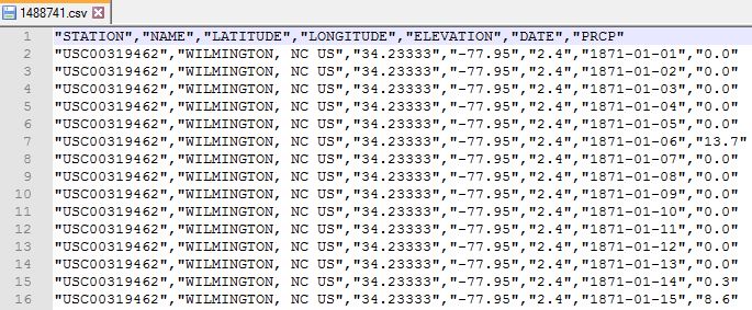
Anyway, once you get an email notifying that the data is ready for download, go ahead and download the CSV files to your working directory. The figure below shows you one such CSV file. I had requested for station information while downloading the data, therefore, in addition to station number (USC00319462) and station name (WILMINGTON, NC US), geographic information such as latitude, longitude, and elevation was also available in the CSV file. The date and precipitation data in mm are the primary columns of interest, which we will analyze further in this article.
Exploratory analysis in RStudio
Open RStudio if you have it installed on your system. Else, use an appropriate R programming interface that is available at your disposal. We will first begin by loading the ggplot2 library required for this exercise and setting the working directory as follows:
library(ggplot2)
setwd("C:/Users/gmallya/Downloads/Hurricane_Florence") # Use your working directory
Next load the CSV file. I have saved the CSV file in a directory inside my working directory.
# Load the CSV file containing daily precipitation data downloaded from NOAA
precip <- read.csv(
  file = "Precip_data/1488741.csv", # File containing precipitation data for USC00319462
  sep=",",
  stringsAsFactors = FALSE
)
The read.csv() function provides an easy way to read CSV files into R. The function attribute file = “Precip_data/1488741.csv” lets R program know the location and the name of the file within the working directory. The sep=”,” attribute specifies the separator used in the CSV file, which is a comma in this case. The stringsAsFactors = FALSE attributes let the read.csv() function know that any “string or character columns” should not be treated as factors. If we do not explicitly set this attribute to FALSE , by default columns such as station number, name, and date may be treated as factors.
The read.csv() function returns a “data.frame” object, which can be checked using the following line of code.
class(precip)
To check if the data has been correctly imported into the data frame, use:
# view first 6 rows of the data frame
head(precip)
To investigate the structure of the data frame, use:
# View the structure (str) of the data frame
str(precip)

###### Expected output
# > str(precip)
# 'data.frame':	29484 obs. of  7 variables:
#   $ STATION  : chr  "USC00319462" "USC00319462" "USC00319462" "USC00319462" ...
# $ NAME     : chr  "WILMINGTON, NC US" "WILMINGTON, NC US" "WILMINGTON, NC US" "WILMINGTON, NC US" ...
# $ LATITUDE : num  34.2 34.2 34.2 34.2 34.2 ...
# $ LONGITUDE: num  -78 -78 -78 -78 -78 ...
# $ ELEVATION: num  2.4 2.4 2.4 2.4 2.4 2.4 2.4 2.4 2.4 2.4 ...
# $ DATE     : chr  "1871-01-01" "1871-01-02" "1871-01-03" "1871-01-04" ...
# $ PRCP     : num  0 0 0 0 0 13.7 0 0 0 0 ...
The output of str(precip), shows that precip data frame has 29484 observations and seven variables. The variables of the data frame are also listed, along with data class (e.g., chr – character, num – numeric, date – date/time etc.) and sample data for each variable.
Plot precipitation data
Next, we will quickly plot the precipitation data using:
# quickly plot precipitation data
qplot(x=DATE, y=PRCP,
      data=precip,
      main="Daily Precipitation\nWILMINGTON, NC US (USC00319462)"
      )
The qplot() function is used to make quick plots. The attributes of the function x=, y=, data= represent the x-variable, y-variable, and the data frame, respectively. The variable and data frame names are case-sensitive. The title of the plot is specified using main=. The title may be split over multiple lines using \n. Go ahead and plot the daily precipitation data using the above code snippet.
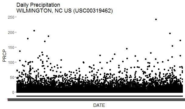
You may have observed that it takes painfully long time (~ 1 minute) to produce a simple plot. Also, the y-ticks and y-tick-labels are unclear! This is because the DATE variable is of class chr. So let us go ahead and explicitly change this to date class.
# convert date column to date class/type
precip$DATE <- as.Date(precip$DATE)
Run the plot code snippet shown below:
# Plot with x- and y-axis labels
qplot(x=DATE,y=PRCP,
      data=precip,
      main="Daily Precipitation w/ Date assigned\nWILMINGTON, NC US (USC00319462)",
      xlab="Date",
      ylab="Precipitation"
      )
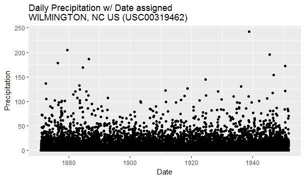
… and voila! Plotting is a breeze! The y-ticks and y-tick-label now properly correspond to years in our data record. We have also correctly labeled the x- and y-axis. Everything looks good, except that the precipitation record at this station is not current. The last date of record is September 30, 1951. You can check this using the tail(precip) command. Nothing to worry at this point. We have at least learned how to read CSV files containing precipitation data into an R data frame and made a quick exploratory plot of precipitation. In the next blog post, we will explore the precipitation time series further – and explore topics such as mass-curve and frequency analysis. Stay tuned, and drop a comment below if you found this blog post useful.
References:
^[1] Scism, Leslie; Aliworth, Erin (21 September 2018). “Moody’s Pegs Florence’s Economic Cost at $38 Billion to $50 Billion”. WSJ. Wall Street Journal